The binomial distribution is, in essence, the probability distribution of the number of heads resulting from flipping a weighted coin multiple times. It is useful for analyzing the results of repeated independent trials, especially the probability of meeting a particular threshold given a specific error rate, and thus has applications to risk management. For this reason, the binomial distribution is also important in determining statistical significance.
A Bernoulli trial, or Bernoulli experiment, is an experiment satisfying two key properties:
A binomial experiment is a series of \(n\) Bernoulli trials, whose outcomes are independent of each other. A random variable, \(X\), is defined as the number of successes in a binomial experiment. Finally, a binomial distribution is the probability distribution of \(X\).
For example, consider a fair coin. Flipping the coin once is a Bernoulli trial, since there are exactly two complementary outcomes (flipping a head and flipping a tail), and they are both \(\frac\) no matter how many times the coin is flipped. Note that the fact that the coin is fair is not necessary; flipping a weighted coin is still a Bernoulli trial.
A binomial experiment might consist of flipping the coin 100 times, with the resulting number of heads being represented by the random variable \(X\). The binomial distribution of this experiment is the probability distribution of \(X.\)
Determining the binomial distribution is straightforward but computationally tedious. If there are \(n\) Bernoulli trials, and each trial has a probability \(p\) of success, then the probability of exactly \(k\) successes is
This is written as \(\text(X=k)\), denoting the probability that the random variable \(X\) is equal to \(k\), or as \(b(k;n,p)\), denoting the binomial distribution with parameters \(n\) and \(p\).
The above formula is derived from choosing exactly \(k\) of the \(n\) trials to result in successes, for which there are \(\binom\) choices, then accounting for the fact that each of the trials marked for success has a probability \(p\) of resulting in success, and each of the trials marked for failure has a probability \(1-p\) of resulting in failure. The binomial coefficient \(\binom\) lends its name to the binomial distribution.
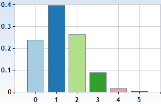
Consider a weighted coin that flips heads with probability \(0.25\). If the coin is flipped 5 times, what is the resulting binomial distribution?
This binomial experiment consists of 5 trials, a \(p\)-value of \(0.25\), and the number of successes is either 0, 1, 2, 3, 4, or 5. Therefore, the above formula applies directly:
\[\begin \text(X=0) &= b(0;5,0.25) = \binom(0.25)^0(0.75)^5 \approx 0.237\\ \text(X=1) &= b(1;5,0.25) = \binom(0.25)^1(0.75)^4 \approx 0.396\\ \text(X=2) &= b(2;5,0.25) = \binom(0.25)^2(0.75)^3 \approx 0.263\\ \text(X=3) &= b(3;5,0.25) = \binom(0.25)^3(0.75)^2 \approx 0.088\\ \text(X=4) &= b(4;5,0.25) = \binom(0.25)^4(0.75)^1 \approx 0.015\\ \text(X=5) &= b(5;5,0.25) = \binom(0.25)^5(0.75)^0 \approx 0.001. \end\]
It's worth noting that the most likely result is to flip one head, which is explored further below when discussing the mode of the distribution. \(_\square\)
This can be represented pictorially, as in the following table:
The binomial distribution \(b(5,0.25)\)
0.00 0.37 0.50 0.63 0.99You have an (extremely) biased coin that shows heads with probability 99% and tails with probability 1%. To test the coin, you tossed it 100 times.

What is the approximate probability that heads showed up exactly \( 99 \) times?
Submit your answerA fair coin is flipped 10 times. What is the probability that it lands on heads the same number of times that it lands on tails?
Give your answer to three decimal places.
There are several important values that give information about a particular probability distribution. The most important are as follows:
Three of these values--the mean, mode, and variance--are generally calculable for a binomial distribution. The median, however, is not generally determined.
The mean of a binomial distribution is intuitive:
In other words, if an unfair coin that flips heads with probability \(p\) is flipped \(n\) times, the expected result would be \(np\) heads.
Submit your answerLet \(X_1, X_2, \ldots, X_n\) be random variables representing the Bernoulli trial with probability \(p\) of success. Then \(X = X_1 + X_2 + \cdots + X_n\), by definition. By linearity of expectation,
\[E[X]=E[X_1+X_2+\cdots+X_n]=E[X_1]+E[X_2]+\cdots+E[X_n]=\underbrace_>=np.\ _\square\]
You have an (extremely) biased coin that shows heads with 99% probability and tails with 1% probability.
If you toss it 100 times, what is the expected number of times heads will come up?
A similar strategy can be used to determine the variance:
Since variance is additive, a similar proof to the above can be used:
\[ \begin \text[X] &= \text(X_1 + X_2 + \cdots + X_n) \\ &= \text(X_1) + \text(X_2) + \cdots + \text(X_n) \\ &= \underbrace_> \\ &= np(1-p) \end \]
since the variance of a single Bernoulli trial is \(p(1-p)\). \(_\square\)
The mode, however, is slightly more complicated. In most cases the mode is \(\lfloor (n+1)p \rfloor\), but if \((n+1)p\) is an integer, both \((n+1)p\) and \((n+1)p-1\) are modes. Additionally, in the trivial cases of \(p=0\) and \(p=1\), the modes are 0 and \(n,\) respectively.
\[ \text = \begin 0 & \text p = 0 \\ n & \text p = 1 \\ (n+1)\,p\ \text< and >\ (n+1)\,p - 1 &\text(n+1)p\in\mathbb \\ \big\lfloor (n+1)\,p\big\rfloor & \text(n+1)p\text< is 0 or a non-integer>. \end \]
Submit your answerDaniel has a weighted coin that flips heads \(\frac\) of the time and tails \(\frac\) of the time. If he flips it \(9\) times, the probability that it will show heads exactly \(n\) times is greater than or equal to the probability that it will show heads exactly \(k\) times, for all \(k=0, 1,\dots, 9, k\ne n\).
If the probability that the coin will show heads exactly \(n\) times in \(9\) flips is \(\frac
\) for positive coprime integers \(p\) and \(q\), then find the last three digits of \(p\).
The binomial distribution is applicable to most situations in which a specific target result is known, by designating the target as "success" and anything other than the target as "failure." Here is an example:
In this binomial experiment, rolling anything other than a 6 is a success and rolling a 6 is failure. Since there are three trials, the desired probability is
\[b\left(3;3,\frac\right)=\binom\left(\frac\right)^3\left(\frac\right)^0 \approx .579.\]
This could also be done by designating rolling a 6 as a success, and rolling anything else as failure. Then the desired probability would be
\[b\left(0;3,\frac\right)=\binom\left(\frac\right)^0\left(\frac\right)^3 \approx .579\]
just as before. \(_\square\)
The binomial distribution is also useful in analyzing a range of potential results, rather than just the probability of a specific one:
In this binomial experiment, manufacturing a working widget is a success and manufacturing a defective widget is a failure. The manufacturer needs at least 8 successes, making the probability
\[ \begin b(8;10,0.8)+b(9;10,0.8)+b(10;10,0.8) &=\binom(0.8)^8(0.2)^2+\binom(0.8)^9(0.2)^1+\binom(0.8)^ \\\\ &\approx 0.678. \ _\square \end \]
This example also illustrates an important clash with intuition: generally, one would expect that an 80% success rate is appropriate when requiring 8 of 10 widgets to not be defective. However, the above calculation shows that an 80% success rate only results in at least 8 successes less than 68% of the time!
This calculation is especially important for a related reason: since the manufacturer knows his error rate and his quota, he can use the binomial distribution to determine how many widgets he must produce in order to earn a sufficiently high probability of meeting his quota of non-defective widgets.
Related to the final note of the last section, the binomial test is a method of testing for statistical significance. Most commonly, it is used to reject the null hypothesis of uniformity; for example, it can be used to show that a coin or die is unfair. In other words, it is used to show that the given data is unlikely under the assumption of fairness, so that the assumption is likely false.
The null hypothesis is that the coin is fair, in which case the probability of flipping at least 61 heads is
\[\sum_^b(i;100,0.5) = \sum_^\binom(0.5)^ \approx 0.0176,\]
or \(1.76\%\).
Determining whether this result is statistically significant depends on the desired confidence level; this would be enough to reject the null hypothesis at the 5% level, but not the 1% one. As the most commonly used confidence level is the 5% one, this would generally be considered sufficient to conclude that the coin is unfair. \(_\square\)